Reverse engineering

The Reverse engineering view of a connection helps to find signals in traffic without a signal database: which bits of an identifier change, how often and when, which bits change when you do something in the vehicle, and what a group of bits looks like as a number over time. Fields you identify can be plotted right away and added to a database.

For diagnostics instead of broadcast traffic, the UDS discovery page finds the services and data identifiers an ECU answers to.

Its tabs:

Tab	Purpose
Bits	The bits and bytes of an identifier, the notch, and the bit field form
Activity	A raster of every bit of one identifier across the whole capture, to see its structure at a glance
Automatic analysis	Checksums, counters, multiplexers, values, states and flags of every identifier, found automatically
Reference signals	The fields following a known value: a database signal, a CSV file (e.g. GPS) or OBD-II values
Markers	The bits changing each time you mark that something happened
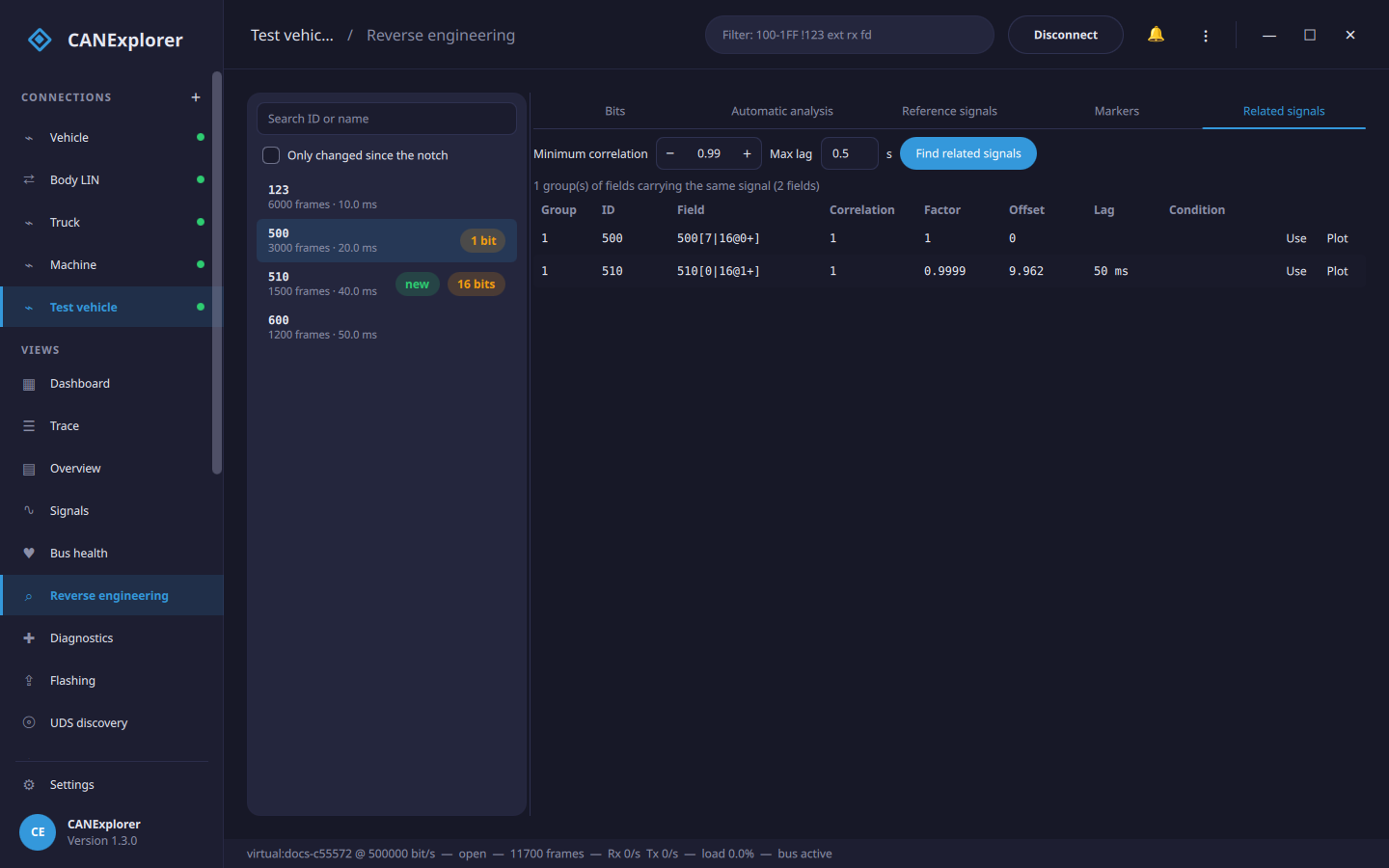
Related signals	Fields carrying the same signal on several messages, grouped
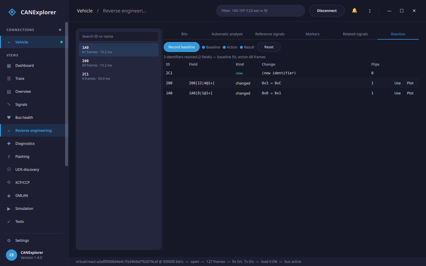
Reaction	Diff a baseline against an action to find what a control or an event changes on the bus
Console	An interactive Python console over the captured frames, with the reverse-engineering primitives

The view works on live buses and on replayed log files. The bit statistics start when it is first opened, including the frames already in the trace, and follow the bus from then on; Clear in the trace toolbar and Reset start again. The other tabs work on the newest million frames of the trace when you start them.

Identifiers

The list on the left shows every identifier with its frame count, cycle time and the message name when a database describes it. Select one to see its bits and bytes.

Bits

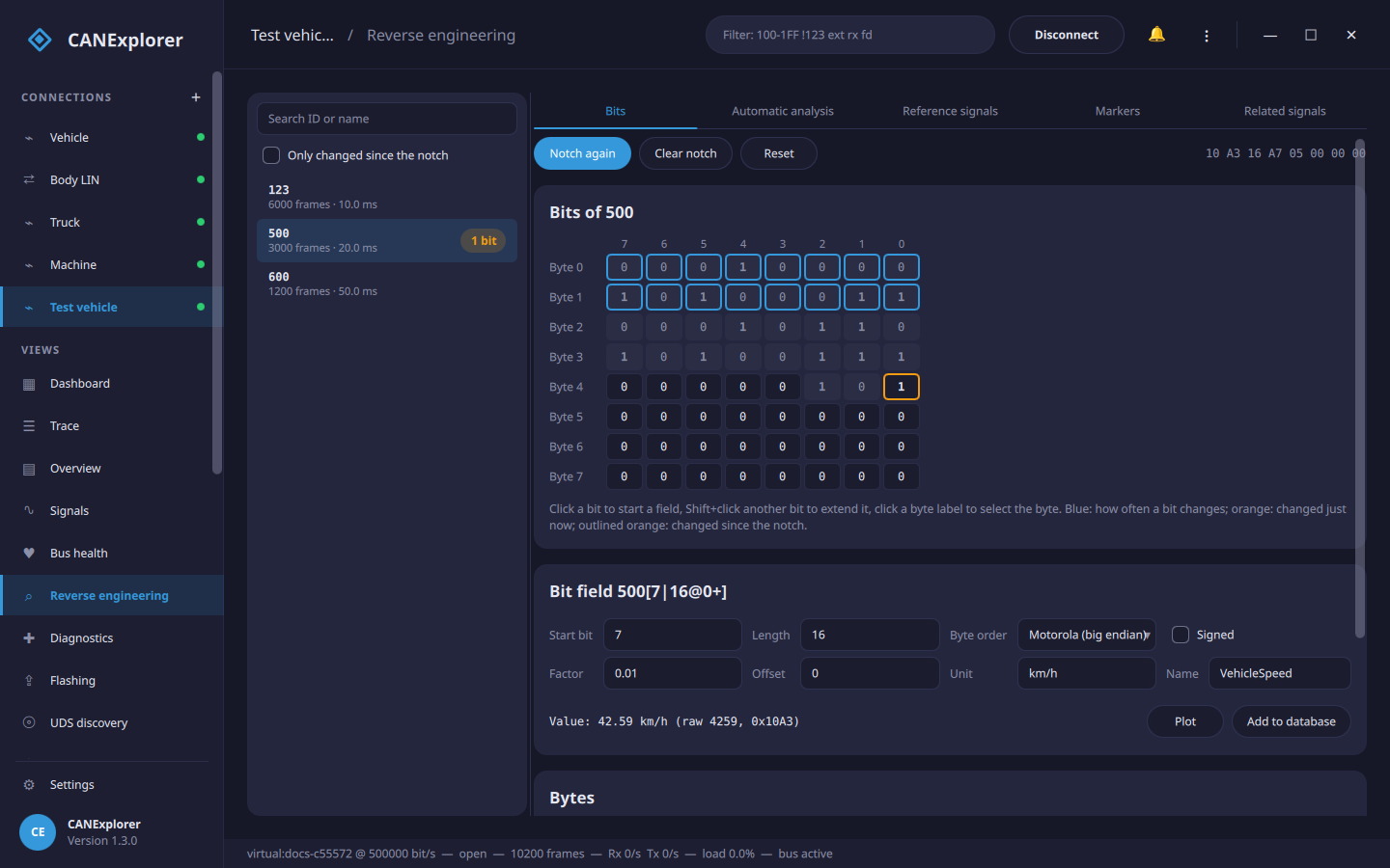
The bit grid shows the bits of the selected identifier as in a DBC file: one row per byte, bit 7 on the left.

• The number in a cell is the bit's value in the last frame.
• Blue cells change; the stronger the tint, the more often (on a logarithmic scale, so a bit changing in one frame in a thousand is still visible). Grey cells never changed.
• A cell flashes orange when the bit changes and fades out over a second.
• The tooltip gives the share of the frames with the bit set, the share of the frames in which it changed, and when it last changed.

Counters show up as a staircase: the lowest bit changes in every frame, the next one in every second frame and so on. Physical values such as speeds look similar but slower and less regular, and flags change rarely.

Temporal replay (scrubbing)

Replay in the Bits toolbar plays the selected identifier's captured frames back over time. A scrubber bar appears: drag the slider to any moment, or press play to watch the frames stream by. While replaying, the bit grid, the byte values and the bit field value show the payload at that moment, and bits that just changed light up and fade — so you can watch the data flow and catch exactly when and how bits move.

• Play / pause runs the capture at its recorded pace; Speed scales it from 0.1× to 10×.
• « and » step one frame back or forward; the slider and the frame N / M readout show where you are.
• Scrub to the instant something happened and read off which bits and bytes changed into it.

Leave replay (toggle Replay off, or select another identifier) to return the grid to the live, latest frame.

Activity map

The Activity tab shows a bit-transition raster of the selected identifier: every bit of its payload across the whole capture at once, so its structure jumps out where the frame-at-a-time grid and replay cannot show it. Each row is a bit (byte 0 at the top, the most significant bit of each byte first) and each column is a frame over time; Refresh rebuilds it from the frames captured so far.

A cell is blue for a steady 1, dark for a steady 0, and orange where the bit changed. The patterns name themselves:

• a counter ramps as diagonal stripes, its low bits busier than its high bits;
• a constant byte is flat (dark or blue);
• a physical value drifts, its high bits slow and its low bits noisy;
• a toggle (a flag, a blinker) is a column of orange that comes and goes;
• a multiplexer switches whole regions of the payload on and off.

Read off which bytes carry something and what kind, then switch to Bits to define the field or Automatic analysis to have it found.

Timing graphs

Two buttons in the Bits toolbar plot the selected identifier on the Signals page, from the frames in the trace so far on:

• Plot Δt graphs the inter-frame interval (the time between consecutive frames, in milliseconds) over time. A flat line is a cyclic message; steps and spikes reveal gateways, bursts and event-triggered messages (a frame sent only when something happens). The cursors, statistics (min/max/mean interval) and CSV export of the signal plots all apply.
• Plot bytes graphs each payload byte as a value over time, one chart per byte — a quick look at which bytes move and how, without defining a bit field first.

Finding the bits of an action: the notch

1. Let the traffic run for a while without doing anything, so that the bits that change by themselves are counted.
2. Press Notch. Every bit that changed so far is hidden (dimmed).
3. Do the action, e.g. press a button, open a door or switch on the lights.
4. Bits that change now are outlined in orange. The identifiers with such bits show how many (e.g. 2 bits), identifiers that appeared only after the notch are marked new, and Only changed since the notch shows just those.

Press Notch again to hide these bits as well (e.g. to separate two buttons), and Clear notch to show all bits again.

Tip

A slowly changing value can reach bits it did not use before the notch (e.g. the upper bits of the engine speed when you accelerate), and these bits stand out too. Keep the rest of the vehicle as steady as possible while doing the action, and repeat it a few times: the bits of the action change every time.

Bytes

The table below the bit field gives for each byte its value in the last frame, how many distinct values it had, its minimum and maximum, its entropy (0 bits: constant, 8 bits: every value equally often) and a histogram of its values from 00 to FF.

Bit fields

A bit field is a group of bits read as a number, like a signal in a database:

• Click a bit in the grid to start a field there, and Shift+click another bit to extend the field to it. Click a byte label to select the whole byte.
• Byte order: Intel (little endian) fields start at their least significant bit and continue upwards, so a 16 bit value with its low byte first spans byte 0 and byte 1. Motorola (big endian) fields start at their most significant bit; a 16 bit value with its high byte first spans byte 0 bit 7 to byte 1 bit 0. Choose the byte order before selecting the bits.
• Signed reads the field as a two's complement number; Factor and Offset convert it to a physical value (value = raw × factor + offset), with a Unit.

The title shows the field in DBC notation, e.g. 1A0[16|8@1+] (start bit, length, 1 Intel or 0 Motorola, + unsigned or - signed), and the value in the last frame is shown below the form.

Plot shows the field on the Signals page, with its values in all frames of the trace so far, next to database signals. A smooth curve means the field is right; a curve jumping between two ranges usually means the byte order, the signedness or a boundary is wrong. Plotted fields are saved in workspaces, and stay when a database is unloaded.

Add to database adds the field as a signal to the database editor, together with a message for the identifier when the database has none (named Message_1A0), and opens the editor. Without a database open in the editor, the connection's database is opened, or a new one started. Save the database and load it into the connection to decode the signal everywhere.

Automatic analysis

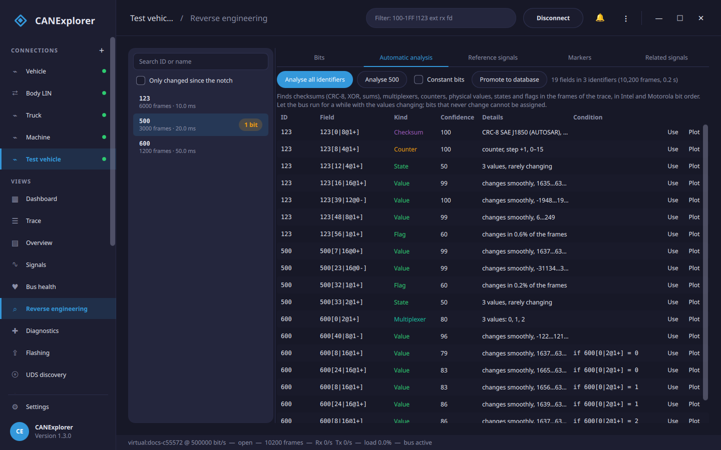
Analyse all identifiers (or only the selected one) looks at the frames of each identifier and lists the fields it finds, with their kind and how sure it is:

Kind	How it is recognised
Checksum	A byte that is a CRC-8 (SAE J1850 / AUTOSAR, 8H2F, SMBus, Maxim, CDMA2000), XOR or sum of the other bytes, with any start value, final XOR, data ID or added constant; also AUTOSAR E2E profile 2 style data IDs depending on a counter
Counter	Changes by the same step from frame to frame and runs through its whole range (alive counters)
Multiplexer	A byte or nibble taking a few values: grouping the frames by its value makes many other bits much calmer. The fields are then found per multiplexer value and shown with their condition, e.g. if 600[0\|2@1+] = 1
Value	Changes smoothly (physical values: speeds, temperatures, voltages); signed when that is smoother, i.e. when it crosses zero
State	A few values, rarely changing (gear, mode)
Flag	A single bit
Constant	Bits that never changed (shown with Constant bits)
Unknown	Changes irregularly: noise, or several fields that could not be told apart

Field boundaries come from how often each bit changes: within a field, the less significant a bit, the more often it changes, so a bit changing much less often than the one above it starts a new field. This is done in both Intel and Motorola bit order, and fields next to each other are told apart by whether one part changes only when the other wraps around (one field) or independently (two fields). As messages normally use one bit order, the bit order giving the more plausible fields is kept.

Getting good results

The analysis can only find bits that change. Record while the values move through a good part of their range (drive, accelerate, steer, switch things on and off) for a minute or more. Bits that never change are reported as constant, so a value that never went negative is found as unsigned, and one that stayed below 256 as 8 bits.

Use shows a field in the Bits tab (for a multiplexed field with its condition, see below); Plot plots it on the Signals page right away.

Promote to database turns the whole result into a draft database in one step: every found field except the constant bits becomes a signal in the database editor, each message is created as needed, and each field's kind, multiplexer condition and details are kept as the signal's comment. Where two interpretations claim the same bits, the more confident one is used, so the signals never overlap. It is a starting point to review — rename the signals, set units and scaling, drop what is noise — and then Save as a .dbc file.

Reference signals

When you know a value from elsewhere, the field carrying it can be found by comparing:

• Database signal: a signal of the connection's database, e.g. to find the same value in another message or on another bus (its own message is left out).
• CSV file: a file with the time in seconds in the first column and values in the others, for example from a GPS logger or a data logger. Headers like speed [km/h] give the unit (the CSV export of the signal plots has this layout). Times below 10⁹ are taken as seconds from the first frame of the trace, larger ones as absolute timestamps.
• OBD-II values (live connections that can transmit): choose values such as the engine speed or vehicle speed, and Start polling while you record. The OBD-II service 01 requests go to the functional address 7DF (18DB33F1 with 29 bit identifiers) one after the other, and the answers become references.

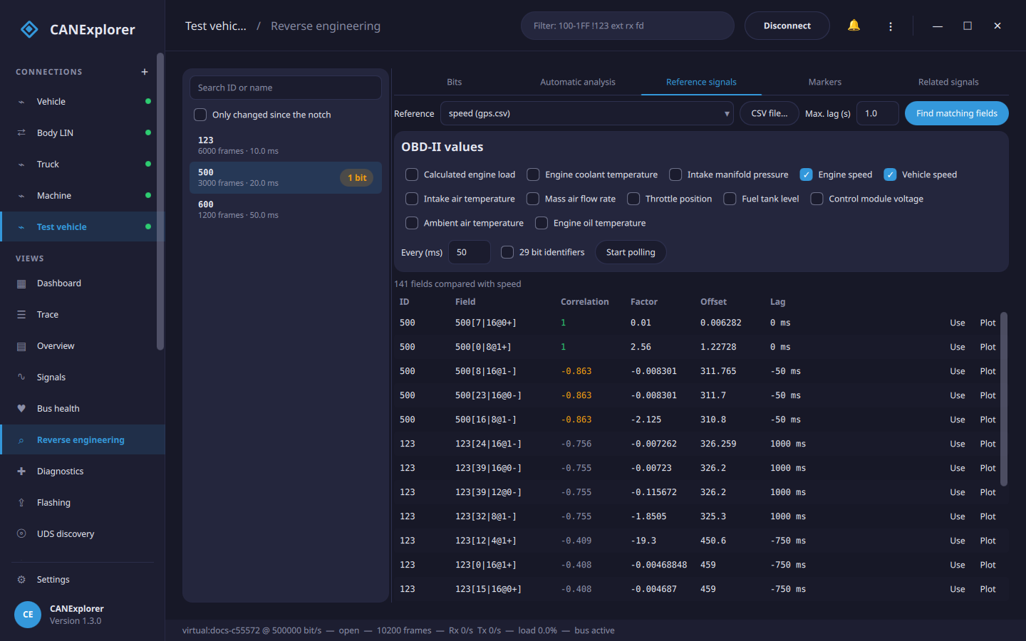
Find matching fields samples every field candidate (the fields of the automatic analysis, and every byte aligned 8 and 16 bit field in both bit orders, unsigned and signed) at the times of the reference and ranks them by their correlation with it. A straight line fit gives the factor and offset converting the field into the reference's unit, and the lag is the delay between them (up to Max. lag) giving the best match. Correlations near 1 (or −1) are good matches; when no field comes close the view says so: the value may not be on this bus, or it was too steady while recording. Use fills the bit field form with the factor, offset, unit and a name.

OBD-II requests

Polling sends diagnostic requests on the bus. Only poll on a vehicle you may send to, and stop when you are done. The requests and answers (7DF, 7E0–7EF, 18DB33F1, 18DAF1xx) are left out of the analysis.

Markers

Markers tell the view when something happened, so the bits changing at that moment can be found, also when they are not the only bits changing:

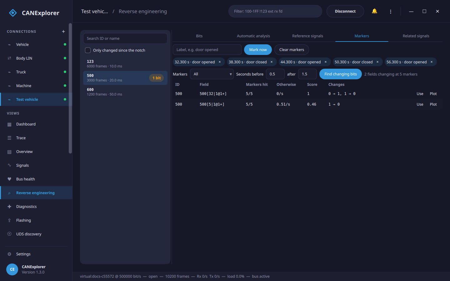
1. Type a label, e.g. door opened, and press Mark now (or Ctrl+M) each time you do the action, e.g. five times opening the door. Several labels can be used, e.g. door opened and door closed.
2. Find changing bits (for all markers or those with one label) lists the fields whose bits changed within the window around most markers (Seconds before and after the marker, so a marker set a little late still counts) but rarely otherwise. Markers hit shows at how many markers, Otherwise how often the bits change elsewhere, and Changes the values before and after, e.g. 0 → 1.

The time of a marker is that of the newest frame, so markers also work while replaying a log file at normal speed.

Related signals

Vehicles often carry the same quantity on several messages — a gateway re-broadcasts wheel speed, engine speed or a pedal position from one bus onto another, sometimes scaled or delayed. Related signals finds these without any reference: every value and state field found by the automatic analysis is compared with all the other fields, and those that follow one another are grouped.

Find related signals lists the groups. Each group's first field is the reference the others are compared with; every other member shows its Correlation to it, the Factor and Offset converting its raw value to the reference's, and the Lag (how far it trails the reference, e.g. a gateway re-broadcasting after 20 ms). Minimum correlation sets how closely two fields must match to be grouped, and Max lag how far apart in time a copy may be.

This labels unknowns cheaply: once one member of a group is identified (here, or against a database or GPS log in Reference signals), the others are the same signal elsewhere. Use a member to load it into the bit field form, or Plot it.

Capture reaction

Reaction answers "I did X — what changed?" the safe way: it records the bus while steady, then while you perform an action, and diffs the two. It never transmits — it only watches — so it is the right tool for finding which message controls something (a relay, a light, a door) without sending unknown frames at the vehicle.

1. Record baseline — leave the bus steady (do nothing) for a few seconds.
2. Start action — now perform the action (press the button, open the door) once.
3. Capture reaction — the action window is diffed against the baseline.

The results list, most reactive first:

• new identifiers that appeared only during the action (an ECU started transmitting), and
• changed fields: runs of bits that were stable throughout the baseline but changed during the action, with their Change (value before → after) and how many times they flipped.

Fields that were already moving on their own during the baseline (counters, live sensors) are left out, so what remains is what the action caused. Use a result to load it into the bit field form, or Plot it.

Having found the controlling message, confirm it by replaying that captured frame back onto the bus with Replay to bus… or the transmit panel — replaying a real, observed message, not a guessed one.

Scripting console

The Console tab is an interactive Python console over the frames captured so far — an ad-hoc frame processor or field hunt with the same primitives the tools use, for when a point-and-click tool does not cut it. Type a snippet in the syntax-highlighted editor and press Ctrl+Enter (or Run); the value of a trailing expression is shown like a Python REPL, print() output is captured, and errors are reported instead of raised. Variables persist between runs; Clear empties the transcript and forgets them. Type HELP for the available names.

In scope:

• messages — the captured frames (can.Message); frames — collect(messages), keyed by (id, extended); analyses and fields — the results of the Automatic analysis tab.
• Helpers ids() and frames_of(id) (the identifier as an int or a hex string).
• The can_explorer.core.reverse primitives: collect, analyse, analyse_all, BitField, candidates, signal_groups, correlate and read_reference_csv.

For example, [(f.field.key, f.kind) for f in analyse(frames_of('100')).fields] lists the fields found in 100, and {hex(i): len(f.payloads) for (i, e), f in frames.items()} counts the frames of each identifier. This is the same scriptable surface the MCP interface exposes to an AI agent, at the keyboard.

Note

The console runs Python in the application's own process — it is not a sandbox. It is for exploring your own capture, so do not paste scripts you do not trust.

Multiplexed fields

A field found for one multiplexer value carries a condition: the bit field form shows only if 600[0|2@1+] = 1, and plotting it takes only the frames with that multiplexer value. Click the condition to use all frames again. Add to database adds the field as a plain signal with the condition in its comment.

Trying it without a vehicle

tools/synthetic_traffic.py writes a log file with traffic from a signal database, with smooth, constant, counting, toggling or noisy signals, and steps at given times:

uv run python tools/synthetic_traffic.py examples/simulation/vehicle.dbc traffic.asc --duration 30 \
    --behaviour EngineData.GearPosition=step:10

Replay traffic.asc at normal speed, open Reverse engineering, select 100, press Notch before 10 seconds and watch bits 24 to 27 when the gear position changes. Then run the automatic analysis: it finds the engine speed, coolant temperature and wheel speed fields, and the gear position as a state.

The tests use tests/data/reverse.dbc (a CRC, an alive counter, Intel and Motorola values, signed values, flags and a multiplexer) with the same generator, and check that the analysis finds every field whose bits change.